Visual Social Network Analysis in R and Gephi Part II
Resuming from last time, I've made some updates to the philosophers' social network including publishing two interactive maps. Quick introduction: you know that sidebar on wikipedia where it tells you someone was influenced by someone else, linking to them? These graphs are generated from asking wikipedia for a comprehensive list of every philosopher's influence on every other. There are some sample-bias issues and data problems I went over in the first part of the series, but overall it's both beautiful and interesting.
Interactive visuals
The first lets you zoom dynamically and makes it easier to see local networks. When you hover over individual philosophers, those who are not linked to them or from them disappear. This uses a tool called sigma.js.
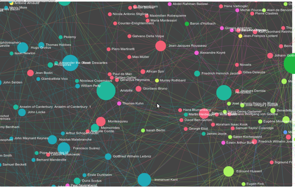
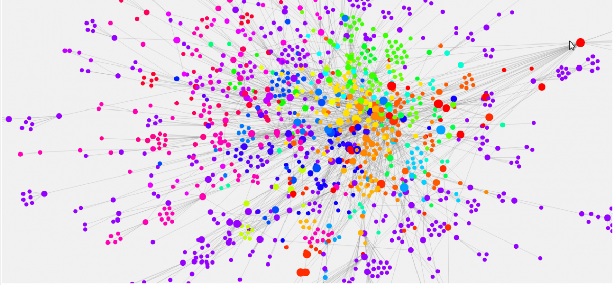
The second lets you actually grab nodes and move them around. This might seem superfluous, but is surprisingly rich in how it lets you see the connected mass of the network---if you move a highly connected node who is also a major hub for different communities---like Hegel---and you'll see the entire graph react immediately. Move someone central, but deeper within a single community---like Hume---and you'll fnd the motions of the graph take some time to propagate outward. It'll move, but the speed it moves at is telling of a different kind of connectedness. This visualization uses a tool called D3 by Mike Bostock.
Moral of the story
The first graphs were pretty, but interactivity is a pretty big deal. It's more than adding another dimension to your plot---it fundamentally changes how you can interact with information. It's the difference between a lecture and a conversation.
Live world tour (of Chicago) ...one day only.
I'm presenting this general topic at the Chicago R User Group's meetup October 3rd. I'll post my slides here once they're finished.
Next up
Stay tuned for Part III, where we'll go over the guts of different influence measures and layouts, what they mean and how to code them. In Part IV, we'll talk about some real life applications in finance (counterparty risk) and marketing.
And the code
# Resuming from last time...
# Write the file (you can import this to gephi)
write.csv(edges,file="Edge_file.csv", row.names=F)

# From http://theweiluo.wordpress.com/2011/09/30/r-to-json-for-d3-js-and-protovis/
toJSONarray <- function(dtf){
clnms <- colnames(dtf)
print(clnms)
name.value <- function(i){
if(class(dtf[, i])!='numeric'){
quote <- '"'
paste('"', i, '":', quote, dtf[,i], quote, sep='')
} else {
paste('"', i, '":', as.numeric(dtf[,i]), sep='')
}
}
objs <- apply(sapply(clnms, name.value), 1, function(x){paste(x, collapse=',')})
objs <- paste('{', objs, '}')
res <- paste('[', paste(objs, collapse=', '), ']')
return(res)
}

##########################################
# Prepare the JSON strings
nattr <- list.vertex.attributes(sg)
eattr <- list.edge.attributes(sg)

name <- get.vertex.attribute(sg, nattr[1])
label <- get.vertex.attribute(sg, nattr[2])
color <- get.vertex.attribute(sg, nattr[3])
pagerank <- as.numeric(get.vertex.attribute(sg, nattr[4]))
size <- as.numeric(get.vertex.attribute(sg, nattr[5]))
katz <- as.numeric(get.vertex.attribute(sg, nattr[6]))
nodelist = data.frame(name,label,color,pagerank,size,katz, stringsAsFactors=FALSE)

source <- as.numeric(get.edgelist(sg, names=F)[,1])
target <- as.numeric(get.edgelist(sg, names=F)[,2])
value <- as.numeric(get.edge.attribute(sg,eattr[1]))
edgelist <- data.frame(source,target,value, stringsAsFactors=F)

# Nest these together (by hand), and this is the input for the D3 visualization
x <- toJSONarray(nodelist)
write(x, 'nodelist.json')
y <- toJSONarray(edgelist)
write(y, 'edgelist.json')

# This is one way of outputting to the sigma.js visualization, but it's probably best to go through gephi first.
ids <- seq(1,length(label)[1])-1
id <- ids
label <- label
idlist = data.frame(ids,label,stringsAsFactors=F)
nodeattr = data.frame(id,nodelist[,c(3,4,5,6)], stringsAsFactors=FALSE)

gexf(nodes=idlist, edges=edgelist, nodesAtt=nodeattr, output="philo.gexf", defaultedgetype = "directed")