Beard line: Time Series in R (Part III)

In Part 2, we showed how to add recession shading to a plot of American Beards over time, and did some diagnostics to check whether 19th Century Americans grew recession beards. (Spoiler alert: it appears they did not.)  In Part 1, we showed how to plot the series in the first place.  Today, we're going to look at the beardly trend over the period.  We all know about the gilded age popularity of mutton chops and sideburns, but were full beards on the rise or on the decline between 1866 and 1911?  And more importantly, what can this period tell us about beards of the future (in the past)?!

What you'll learn

• How to apply linear smoothing to a time-series plot in ggplot2
• How to interpret that and how not to interpret that.  (The difference between interpolation and extrapolation.)
• Whether beards were getting "trendier" or trending less during the tail end of the 19th Century.
• What date we're all going to have beards.

The Data

As before, the data comes from...

Robinson, D.E. Fashions in shaving and trimming of the beard: the men of the Illustrated London News, 1842-1972. American Journal of Sociology, 81:5 (1976), 1133-1141.

...via the TSDL.

The recession dates come from the NBER.

Let's Take a Look

We don't have much to add from the previous example.  In fact, you only need to put a single line onto the previous script:

# Add a bearded trend line
bplot3 <- bplot2 + geom_smooth(se=F, method="lm", formula=y~x, colour='red', size=1.125)
print(bplot3)

This provides a linear trend (method="lm"),  removes the standard error bands (se=F), asks for a linear regression to be applied (y~x), and colors the line red.

Some Notes

• If you had to characterize all the points on the chart with only a single line, which line would that be?  The command "formula=y~x" in the function above asks for a line that minimizes the sum distance between all points and our estimated line---it's a linear regression, the unique line through our dataset that minimizes how far away our observations are from our estimate.  What's subtly impressive about this is that there's only one such line that solves this optimization problem (for most well behaved 2-variable data you'll encounter). Try as you can, even with the best ruler and sharpest eyes, you won't be able to draw a better fitting line.
• What does it tell you?  It says that over the period, if you had to bet whether beardfullness was increasing or decreasing, you'd want to say increasing--and tells you by how much, on average, from year to year.  This line is a model or a simplification for beardfulness over the whole sample period, without having to write down all the data points.  So, if I threw out all the data that made this chart, but still had this line, I'd have a very concise summary.  All you'd have to do is tell me the year, and I could plug it into the starting value, the slope, and have an estimate of American beardfulness.  That's parsimony.
• However, this is actually a horrible estimate, because it doesn't use enough conditional information, which is where stationarity in time series analysis comes in.  More on that in Part IV.

For now...

Beautiful Results

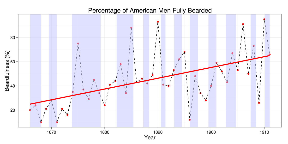
You can see our estimate, the red line, shows that in general, there was a trend of increasing beardfulness in late 19th Century America.

A Little more

The line we drew is a way of simplifying the information within our sample.  It lets us construct new estimates in-between years, even.  (Well, a second way---we've already done that once with the dotted lines between points.)  In-sample estimation is called interpolation.  You'd contrast that with extrapolation---which is estimating points beyond our sample. As you can see, the linear model interpolation is not spectacular---there are times when the sample deviates quite far from the intermediate value line we drew, and where using it would result in a bad estimate.

Well, extrapolating from this unfit model would be even worse.  It's bad enough that we should try it, as a motivatation for how we can do better.  So, let's extend this linear model into the future.  Let's forecast, and extrapolate from our model fit until we hit...

Peak Beardfulness

Our model is a simple line.  It never changes direction.  If it started up, over enough time, it'll go up to infinity.  If it started pointed down, it would just always get more negative.  So if we see it continuing up within our sample---there must be a time outside and beyond our sample when our line hits 100% and never turns back.  That is, our model suggests the shocking conclusion that we will someday hit 100% beardfulness.

When?

Using the following code from the "forecast" package in R, we can find the very year in which American beardfulness reaches 100%.

fit <- lm(data=beard.df,beard~date) # Fit a linear model
fdates <- as.Date(timeSequence(        # Over the next 100 years
    from = "1912-01-01",
    length.out = 100,
    by = "year"))
new <- data.frame(date=fdates)     # Make a new data frame
pred <- predict(fit,newdata=new) # Extrapolate over the new period
fcast <- cbind(new,pred)     # Connect past to future
names(fcast) <- c("date", "beard")
print(first(fcast[fcast$beard>100,])[,1]) # Stop at 100%...

The output of the forecast says the first date where our forecast exceeds 100% is in 1951.  Excellent.  Problem solved.

(Here is some Evidence we did not hit peak beard in 1951.)

What Went Wrong?

If you've ever looked around at modern American faces---generally unless you're looking at elderly math professors or the homeless--you'll know the answer is that we do not reach 100% beardfulness, but that beardfullness actually decreases in post-war America.  This is an illustration of the failure of extrapolation from an unsuitable model, right?---or perhaps it's a failure of American beardfulness...

You could actually argue both---on the one hand, our model didn't fully capture all the information in the data that would have given us better estimates. But on the other hand, something else was happening---trends changed.  In response to cultural fashions not present in the original data, previous data was no longer relevant---there was a regime change in beard standards that couldn't be foreseen within the previous data set---even if you could extract all the information from it, the rise of this trend likely just didn't exist or provide a signal beforehand.  Even with the best of models, the relationship between variables can change over time.

So, how can we do better?  Well...

Next up

We'll add credits to our plot for pretty publication and also explore why time series stationarity matters in making better forecasts.