Recession Beard? Time Series in R (Part II)

In Part I, we showed how to plot a time series of the change in American beards over time, using a dataset from Robert Hyndman's time series data library.  Today, we're going to look at whether the dramatic changes in American male beardfulness seem related to the economy.  Did Americans grow recession beards in response to the Panic of 1873?  Out of work, did they forgo their frequent trips to the barber (since Gillette didn't invent the personal safety razor until 1904 so they could do it themselves)?  Did they go on their job interviews with a face full of mutton chops and just never get called back (by telegram)?

What you'll learn

• How to apply recession shading, according to the NBER's recession dates, to a time series---easily.
• How to change the color of the recession shading
• Whether 19th century gentlemen grew recession beards after losing their jobs in algo trading, you know, just taking some time off to study graphic design for a little bit.

The Data

As before, the data comes from...

Robinson, D.E. Fashions in shaving and trimming of the beard: the men of the Illustrated London News, 1842-1972. American Journal of Sociology, 81:5 (1976), 1133-1141.

...via the TSDL.

The recession dates will come from the National Bureau of Economic Research's Business Cycle Dating Committee (it's like OKCupid but for economists who ride Schwinns).

Parsing this file and applying these dates could be more difficult, but luckily the tis package, maintained by Jeff Hallman, does the heavy lifting for you.

Let's take a look

Here's the code that will produce our plot.

library(XML)         # read.zoo
library(xts)         # our favorite time series
library(tis)         # recession shading.
library(ggplot2)     # artsy plotting
library(gridExtra)   # for adding a caption
library(timeDate)    # for our prediction at the end

# Get the data from the web as a zoo time series
URL <- 'http://robjhyndman.com/tsdldata/roberts/beards.dat'
beard <- read.zoo(URL,
    header=FALSE,
    index.column=0,
    skip=4,
    FUN=function(x) as.Date(as.yearmon(x) + 1865))
# Last line is tricky, check here:
#http://stackoverflow.com/questions/10730685/possible-to-use-read-zoo-to-read-an-unindexed-time-series-from-html-in-r/10730827#10730827

# Put it into xts, which is a more handsome time series format.
beardxts <- as.xts(beard)
names(beardxts) <- "Full Beard"

# Make into a data frame, for ggplotting
beard.df <- data.frame(
    date=as.Date(index(beardxts),format="%Y"),
    beard=as.numeric(beardxts$'Full Beard'))

# Make the plot object
bplot <- ggplot(beard.df, aes(x=date, y=beard)) +
    theme_bw() +
    geom_point(aes(y = beard), colour="red", size=2) +
    ylim(c(0,100)) +
    geom_line(aes(y=beard), size=0.5, linetype=2) +
    xlab("Year") +
    ylab("Beardfulness (%)") +
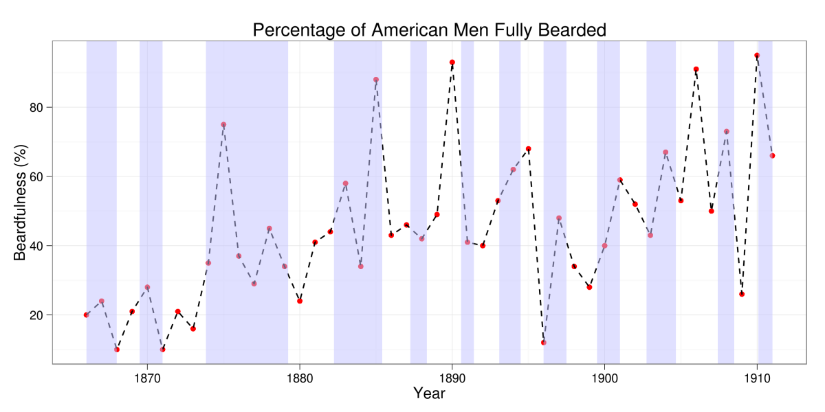
    opts(title="Percentage of American Men Fully Bearded")
print(bplot)

# Add recession shading
bplot2 <- nberShade(bplot,
    fill = "#C1C1FF",
    xrange = c("1866-01-01", "1911-01-01"),
    openShade = TRUE) # looks weird when FALSE

#Plot it
print(bplot2)

Some Notes

• The default recession color is a shade of light grey, which already looks great for recession shading.  However, I changed the color to a light blue because a forecast we're going to do later has grey error bands.
• xrange lets you set the recession to go a bit beyond your actual plot.  As you can see, our sample begins and ends during recessions.  So, if you changed these limits, you could see the full duration of those periods.
• Eyeballing this, I'd say there's no relationship between recession and American beardfulness, unfortunately.

Beautiful Results

A little more

Just looking at it, I can't tell for sure whether there's any relationship between beards and recessions.  It seems to go up and down independently of whether it's in the blue shade or not.  But we can try a couple of simple tests to challenge our hunch.  We're going to start with easy ones and get more sophisticated as we need.

First, let's test whether the average beardfulness during recessions is statistically different from the average beardfulness outside of recessions.  The following code...

1. Identifies which samples are in the recession.
2. Finds the mean amount of beard in-recession and out-of-recession
3. Performs a t-test to test whether these means are the same. This isn't an ideal test for the following reasons....
   • You should check whether the samples are normal first.  Your intuition would tell you they're not because they're percentages. 
   • You should also check that variances are equal.
   • This is a time series, so you might suspect dependence over time, that the samples aren't iid.
   • ...but we're dealing with 19th Century beards here, so we will note this and suspend great methodology for a moment.

Anyway, here is the code:

beardxts$recess <- 0
for (x in seq(1,dim(beardxts)[1])){
  for (y in seq(1,dim(nberDates())[1])){
    if (index(beardxts)[x] >= as.Date(as.character(nberDates()[y,1]),format="%Y%m%d") &
      index(beardxts)[x] <= as.Date(as.character(nberDates()[y,2]),format="%Y%m%d")){
      beardxts$recess[x] <- 1
    }
  }
}

mean(beardxts$Full.Beard[beardxts$recess==1]) # IN-Recession average beard rate
mean(beardxts$Full.Beard[beardxts$recess!=1]) # OUT-OF-Recession average beard rate
x1 <- as.numeric(beardxts$Full.Beard[beardxts$recess==1])
y1 <- as.numeric(beardxts$Full.Beard[beardxts$recess!=1])
t.test(x1,y1)

Your output should be...

[1] 45.5
[1] 44.45833

    Welch Two Sample t-test

data:  x1 and y1
t = 0.1606, df = 43.345, p-value = 0.8731
alternative hypothesis: true difference in means is not equal to 0
95 percent confidence interval:
 -12.03270  14.11603
sample estimates:
mean of x mean of y
 45.50000  44.45833

Interpreting what that's all about

Hypothesis testing can be a little tricky.  What we're testing is whether the average beardfulness level in recession times is the same as in non-recession times.  The test above tells us that the average amount of in-recession beardfulness is 45.5% full-bearded, while the average amount of out-of-recession beardfullness is 44.45% full-bearded---basically the same. 

If you had to be sure, though---say you had to bet on it---how would you define "basically the same?" 

Well, the t-test above tells us that if the average was as low as 32% or as high as 59%, it still would have been close enough that we couldn't say with much certainty otherwise---this whole range is our 95% confidence interval for where we expect the mean to be, based on our sample.  (Note: the difference in true means is non-random, it's the confidence bands that change with the sample.)

Furthermore, since this is a time series, if you wanted to say with certainty, you'd change your test a bit.  Instead of asking whether the level of full-beard is the same, you'd want to check for the rate of change.  That is, because of the fact that we're measuring the same thing over time, and that tomorrow's facial hair is probably dependent on today's, you have what's called serial correlation.  Your samples are not independent over time, and the series is not stationary.  However, your rate of change might be.  More on that later...

Reflections

• At least in the 19th Century, there were no recession beards...
• ...but we'll see how that unfolds when we analyze more rigorously.
• See anything that can be improved?  Leave it in the comments!

Next up...

To characterize "trends" we'll add a line to our graph in Part III.